An Illustration of the SR3 Idea

Sparse Relaxed Regularized Regression — SR3

Regularized regression problems are ubiquitous in the applied sciences, in particular in the fields of statistical modeling, signal processing, and machine learning. Often, a sparsity promoting regularization is used, particularly when a parsimonious representation is desired, as in machine learning-based model discovery. Here, we present the basic idea and a software demonstration of a new approach to such problems: sparse relaxed regularized regression (SR3).

Formulation

Consider a generic linear regression problem

$$\min_{\mathbf{x}}~~\frac{1}{2}\|\mathbf{A} \mathbf{x}-\mathbf{b}\|^2 + \lambda R(\mathbf{C} \mathbf{x}) \, ,$$

where \( \mathbf{A} \) is a measurement matrix, \(\mathbf{b} \) is a signal, and \( R(\mathbf{C}\mathbf{x}) \) is a regularization. For such a problem, SR3 introduces the relaxed coordinates \(\mathbf{w}\) which approximate \( \mathbf{C}\mathbf{x} \), i.e.

$$\min_{\mathbf{x},\mathbf{w}} \frac{1}{2}\|\mathbf{A}\mathbf{x}-\mathbf{b}\|^2 + \lambda R(\mathbf{w}) + \frac{1}{2\eta} \|\mathbf{C}\mathbf{x}-\mathbf{w}\|^2,$$

where \( \eta \) controls the closeness of \(\mathbf{w}\) to \( \mathbf{C}\mathbf{x} \). If you minimize out \( \mathbf{x} \) from the relaxed equation (with any sort of least squares solver), you obtain a problem in \(\mathbf{w}\) alone of the form

$$\min_{\mathbf{w}} \frac{1}{2}\|\mathbf{F} \mathbf{w} - \mathbf{g}\|^2 + \lambda R(\mathbf{w}) \; .$$

where

$$\mathbf{F} = \begin{bmatrix} \kappa \mathbf{A} \mathbf{H}^{-1}\mathbf{C}^\top\\ \sqrt{\kappa}(\mathbf{I} - \kappa \mathbf{C} \mathbf{H}^{-1} \mathbf{C}^\top) \end{bmatrix}, \mathbf{G} = \begin{bmatrix} \mathbf{I} - \mathbf{A} \mathbf{H}^{-1} \mathbf{A}^\top\\ \sqrt{\kappa}\mathbf{C} \mathbf{H}^{-1} \mathbf{A}^\top \end{bmatrix}, \mathbf{g} = \mathbf{G} \mathbf{b}.$$

An important observation is that the properties of \(\mathbf{F}\) are often significantly better than the properties of \(\mathbf{A}\). In particular, \(\mathbf{F}\) generally has a lower condition number than \(\mathbf{A}\). In the image above, we illustrate this idea for the popular LASSO regularizer, i.e. \( R(\cdot) = | \cdot |_1 \) Part (a) shows the level sets (green ellipses) of LASSO and corresponding path of prox-gradient to the solution (40 iterations) in \(x\) coordinates and part (b) shows the level sets (green spheres) of the SR3 value function and corresponding SR3 solution path (2 iterations) in \(w \) relaxed coordinates. Blue diamonds show the \(\ell_1\) ball in each set of coordinates. The \(F\) formulation has a smaller ratio of largest to smallest singular value than \(A\), squashing the level sets into spheres, accelerating convergence, and improving performance.

The relaxed coordinates also suggest a natural algorithm for such problems: proximal gradient descent on the problem in \(\mathbf{w}\) alone. The formulas for \(\mathbf{F}\) and \(\mathbf{g}\) also allow for the use of acclerated methods, e.g. FISTA when \(R\) is the LASSO penalty.

Software Demo — MATLAB Package

The following is a demo included with the SR3 MATLAB package, available on GitHub.

Problem 1: \(\ell_1\) vs \(\ell_0\) penalties

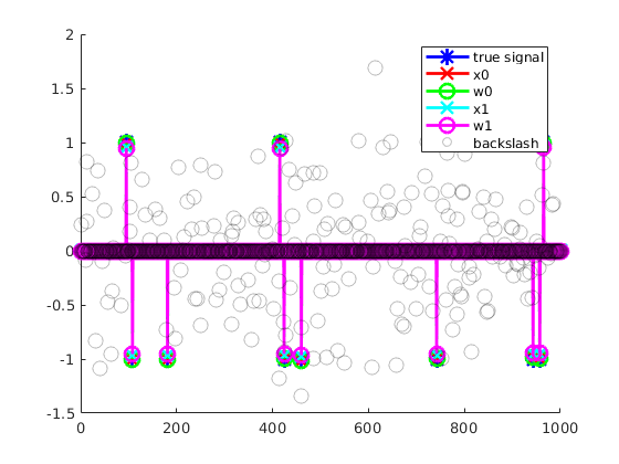
In this problem we test the performance of using SR3 to recover a sparse signal. Here \(R\) is either the \(\ell_1\) or \(\ell_0\) penalty. We also plot the results of a least squares fit and the built in lasso function (if available). This is a relatively easy problem and all of the regularizers perform well, beating the standard least squares approach for obvious reasons.

% matrix dimensions
m = 200;
n = 1000;
k = 10; % number of non-zeros in true solution
sigma = 1e-1; % additive noise

A = randn(m,n);

y = zeros(n,1);
ind = randperm(n,k);
y(ind) = sign(randn(k,1));

b = A*y+sigma*randn(m,1);

% set up parameters of fit
lam1 = 0.01; % good for l_1 regularizer
lam0 = 0.004; % good for l_0 regularizer

% apply solver
[x0, w0] = sr3(A, b, 'mode', '0', 'lam',lam0,'ptf',0);
[x1, w1] = sr3(A, b, 'lam',lam1,'ptf',0);

% built-ins
xl2 = A\b;
if exist('lasso','builtin')
    xl1 = lasso(A,b,'Lambda',lam1);
end

% plot solution
% both regularizers perform well on this problem, though the $\ell_1$
% regularizer introduces a little more bias
figure(); hold on;
plot(y, '-*b'); plot(x0, '-xr'); plot(w0, '-og'); plot(x1, '-xc');
plot(w1, '-om'); scatter(1:length(xl2),xl2,'ok', ...
    'MarkerFaceAlpha',0.25,'MarkerEdgeAlpha',0.25);
if exist('lasso','builtin')
    plot(xl1,'-ok');
    legend('true signal', 'x0', 'w0', 'x1', 'w1','backslash','lasso');
else
    legend('true signal', 'x0', 'w0', 'x1', 'w1','backslash');
end

clear;

Problem 2: regularized derivatives

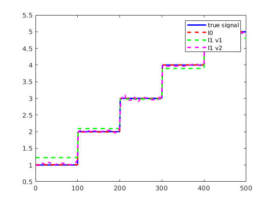
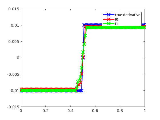
In this problem, we take random projections of a smooth signal and attempt a reconstruction under a piecewise smoothness promoting regularization. Specifically, we assume \(x\) to be a piecewise smooth 1D signal (though the measurements are possibly corrupted by noise). We consider both \(x\) given by a hat function and \(x\) given by a piecewise constant function. We then let \(A\) be an \(m \times n\) random measurement matrix, with \(m < n\). We set up \(C\) to be the \(n-1\times n\) matrix mapping the signal to a finite difference approximation of the derivative. We then reconstruct the signal as the cumulative sum of \(w\), adjusting for the integration constant.

iseed = 8675309;
rng(iseed);

n = 500;
m = 100;
sigma = 0.1;
A = randn(m,n);

% set up signal as step function (sparse derivative assumption)

y = zeros(n,1);
for i = 1:5
	y((i-1)*100+1:i*100) = i;
end

b = A*y + sigma*randn(m,1);

e = ones(n,1);
C = spdiags([-e,e],[0,1],n-1,n); % difference matrix

lam0 = 0.01;
lam1 = 0.02;
lam1_2 = 0.002;

% apply solver
[x0, w0] = sr3(A, b, 'mode', '0', 'lam',lam0,'ptf',0,'C',C);
[x1, w1] = sr3(A, b, 'mode', '1', 'lam',lam1,'ptf',0,'C',C);
[x1_2, w1_2] = sr3(A, b, 'mode', '1', 'lam',lam1_2,'ptf',0,'C',C);

cs = cumsum([0;w0]);
y0 = cs + (sum(x0)-sum(cs))/n;
cs = cumsum([0;w1]);
y1 = cs + (sum(x1)-sum(cs))/n;
cs = cumsum([0;w1_2]);
y1_2 = cs + (sum(x1_2)-sum(cs))/n;

figure()
plot(y,'b')
hold on
plot(y0,'--r')
plot(y1,'--g')
plot(y1_2,'--m')

legend('true signal', 'l0', 'l1 v1', 'l1 v2');

% set up signal as piecewise linear (Chartrand example)
% note that here the regularization is on the second derivative
% also, the regularization is sensitive to lambda

n = 100;

t = linspace(0,1,n).';
tmid = (t(2:end)+t(1:end-1))/2.0;
h = t(2)-t(1);
y = abs(t-0.5);

b = y + sigma*randn(n,1);

bstart = b(1);
b = b-bstart;

sigma = 0.05;

A = tril(ones(n,n-1),-1)*h;
e = ones(n,1);
C = spdiags([-e,e],[0,1],n-2,n-1)/h;

lam0 = 0.007;
lam1 = 0.001;

xi = diff(b)/h;
wi = C*xi;

kappa0 = 1.0*h;
kappa1 = 1.0*h;

% apply solver
[x0, w0] = sr3(A, b, 'mode', '0', 'lam',lam0,'itm',10000,'ptf',0,...
    'C',C,'x0',xi,'w0',wi,'kap',kappa0);
[x1, w1] = sr3(A, b, 'mode', '1', 'lam',lam1,'itm',10000,'ptf',0,...
    'C',C,'x0',xi,'w0',wi,'kap',kappa1);


% reconstruct from w

cs = cumsum([0;w0])*h;
sw0 = cs + (sum(x0)-sum(cs))/length(cs);
sw0int = A*sw0;
coeffs = [sw0int,ones(n,1)]\(b+bstart);
y0 = coeffs(1)*sw0int + coeffs(2)*ones(n,1);
cs = cumsum([0;w1])*h;
sw1 = cs + (sum(x1)-sum(cs))/length(cs);
sw1int = A*sw1;
coeffs = [sw1int,ones(n,1)]\(b+bstart);
y1 = coeffs(1)*sw1int + coeffs(2)*ones(n,1);

figure()
plot(t,y,'b')
hold on
plot(t,b+bstart,'--','color',[0,0,0]+0.75);
plot(t,y0,'--r')
plot(t,y1,'--g')

legend('true signal','corrupted', 'l0', 'l1');

figure()
plot(tmid,diff(y),'-xb')
hold on
plot(tmid,diff(y0),'-xr')
plot(tmid,diff(y1),'-xg')
legend('true derivative', 'l0', 'l1');

Published with MATLAB® R2018a

Links

For more information and to download the software, see

• The preprint on arXiv
• The GitHub repo for the MATLAB package, including some demos and applications.